Other Model Performance Considerations

Fundamental Changes to Business Over Time

In almost every data science problem, the more data, the better. Time series forecasting is one of the few data science problems that has an exception to that statement. To properly adjust this statement for time series, it should be phrased as: the more data, the better… as long as the data patterns remain largely consistent from the beginning of the data history to now.

This means that if the data patterns change wildly over the course of time, the old and outdated data patterns have little to no importance to the data patterns that exist and need to be forecasted now. From a model point of view, blending old and outdated data patterns with new patterns may only lead to confuse the models and lead to bad performance. Examples of this include data sets or businesses that have been heavily affected by the COVID-19 pandemic in 2020, and completely changes the underlying sales patterns and consumer behavior to look nothing like pre-COVID-19.

Long Forecast Ranges Using Daily Data

Long forecast ranges will typically yield lower performance to shorter forecast ranges. This is because there will be more meaningful features able to aid in the prediction when the forecast range is shorter.

Explaining with Lags

In time series forecasting, a target variable is usually heavily correlated with its most recent prior values.

In a daily granularity restaurant sales forecasting example, the sales value today will be heavily correlated with the sales value from 7 days ago. This is because a strong weekly seasonal data pattern found in the data in a daily level data set, today’s (Monday’s) sales value will be correlated with prior values.

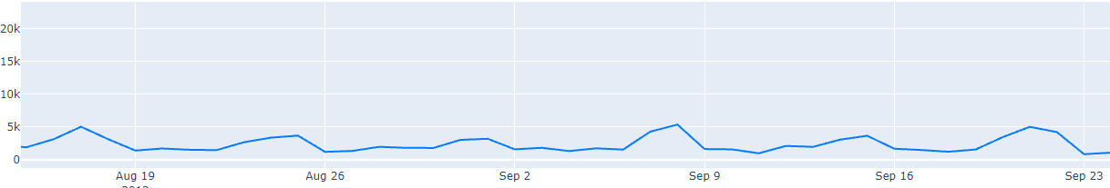
The following graphic shows the daily sales data. There are routine spikes near the weekend. This is weekly seasonality which makes intuitive sense given that this is a restaurant bar that will experience higher sales on the weekend.

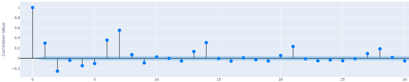
The following auto-correlation plots how correlated each lag of the target variable is with the actual target variable. The 6th and 7th day target lags are highly correlated (.35, .55 respectively) with the target. Additionally, as you move further out, 14, 21, and 28 day target lags are the next highly correlated with the target. The key takeaway is that the further away you get from the actual day (lag days), the less correlated that value is. The smaller the lag number, the more likely the correlation value is high, the more important the lag is an aiding in the prediction of the target.

What do lags have to do with a Long Forecast Range?

In time series, lags of the target variable are powerful features that ultimately lead to a big performance boost. Like the correlation plot shows, a lag feature will typically become less impactful to the model performance the further away you get from the current day.

In time series forecasting, you are forced to lag any features values that you do not know in advance by the length of the forecast range. That means if we want to forecast 21 days ahead on this data set, we can only leverage lags greater than 21 days. Lags of 1, 6, 7, 13, 14, and 20 days will not be able to be used as features in this case. If we were to attempt to produce a 21-day forecast with the previous lags, all of those lags would be missing data necessary to make a prediction.

To summarize:

• The smaller the lag number, the more likely the correlation value is high, the more important the lag is when aiding in the prediction of the target.

• You are forced to lag any features values that you do not know in advance by the length of the forecast range.

Having a large forecast range leads to having less impactful lag features that give lower model performance compared to a short forecast range.

NOTE: Features that are known in advance are features such as events since they happen on a repeated basis. There is no need to lag events.